Introduction
There are many ways in which to increase the realism of a computer generated image. One such method is to calculate the effects of shadowing on an object when evaluating its lighting equations. There is a very wide variety of shadowing techniques available for use in real-time computer graphics, with each technique exhibiting both advantages and disadvantages. In general, shadowing techniques try to strike some balance between shadow quality and runtime performance.
One such technique has been termed Screen Space Ambient Occlusion (SSAO). This technique was originally discussed by Martin Mittring when presenting the paper “Finding Next Gen” at the 2007 SIGGRAPH conference. The basic concept behind the algorithm is to modify the ambient lighting term [see the lighting section of the book for details about the lighting equation :Foundation and theory] based on how occluded a particular point in a scene is. This was not the first technique to utilize the concept of ambient occlusion, but as you will see later in this chapter Screen Space Ambient Occlusion makes some clever assumptions and simplifications to give very convincing results while maintaining a high level of performance.
컴퓨터에서 생성되는 이미지의 현실성을 높이기 위한 많은 방법들이 있다. 이러한 방법중 하나는 조명 방정식을 평가할 때 오브젝트에 그림자 효과를 계산하는 것이다. 실시간 컴퓨터 그래픽스에서 사용할 수 있는 매우 널리 알려진 다양한 그림자 기법들이 있다. 각각의 기법들은 장단점을 가지고 있다. 보통 그림자 기법들은 그림자 퀄리티와 실시간 퍼포먼스 사이에서 약간의 밸런스를 취한다.
이러한 테크닉중 하나는 SSAO라고 한다. 이 기법은 2007 SIGGRAPH 컨퍼런스에서 "Finding Next Gen" 발표때 Martin Mittring에 의해 처음으로 논의되었다. 이 알고리즘의 기본 개념의 배경은 씬에서 특정 점이 얼마나 차폐되었는지를 기반으로 환경광을 수정하는 것이다. [Foundation and Theory에 조명 방정식에 대해서 자세하게 알고 싶으면 책의 조명 부분을 봐라.] 이것은 Ambient Occlusion의 개념을 이용하는 첫번째 테크닉은 아니지만, 이 챕터 나중에 SSAO가 매우 확실한 결과를 주는 반면에 높은 레벨의 퍼포먼스를 내기 위해 얼마나 영리한 가정과 단순화를 했는지 알게 될 것이다.
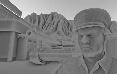
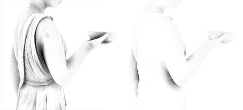
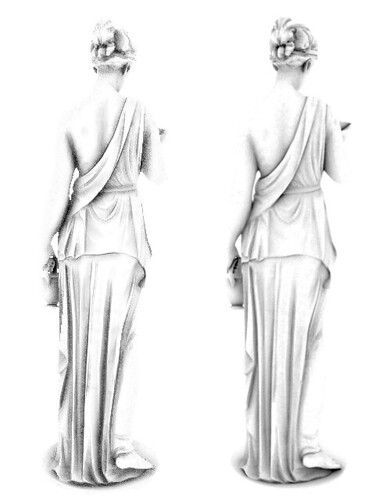
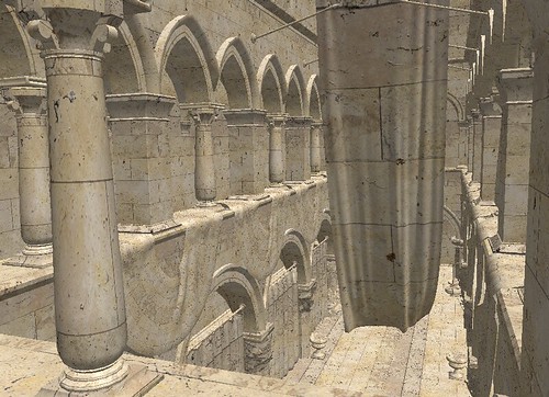
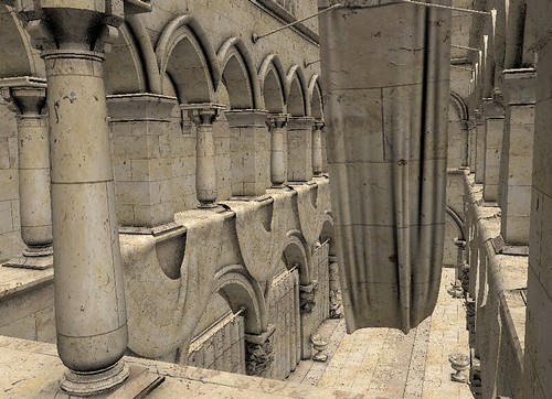
 Figure 1: Sample rendering utilizing screen space ambient occlusion.
In this chapter, we will explore the theory behind the Screen Space Ambient Occlusion technique, provide an implementation of the technique that utilizes the Direct3D 10 pipeline, and discuss what parameters in the implementation can be used to provide scalable performance and quality. Finally, we will discuss an interactive demo which uses the given implementation and use it to give some indication of the performance of the algorithm.
이 챕터에서 우리는 Direct3D 10 파이프라인을 사용하는 구현을 제공하여 SSAO 기법의 뒤에 깔린 이론을 알아볼 것이고 구현에서 어떤 인자들이 재볼 수 있는 퍼포먼스와 퀄리티를 제공하는데 사용되는지 의논할 것이다. 마지막으로 우리는 주어진 구현을 사용하는 데모에 대해 의논하고 알고리즘의 퍼포먼스의 징후를 보는데 사용할 것이다.
Algorithm Theory
Now that we have a background on where screen space ambient occlusion has come from, we can begin to explore the technique in more detail. SSAO differs from its predecessors by making one major simplification: it uses only a depth buffer to determine the amount of occlusion at any given point in the current scene view instead of using the scene information before it is rasterized. This is accomplished by either directly using the depth buffer or creating a special render target to render the depth information into. The depth information immediately surrounding a given point is then scrutinized and used to calculate how occluded that point is. The occlusion factor is then used to modify the amount of ambient light applied to that point.
The generation of an occlusion factor using the SSAO algorithm is logically a two step process. First we must generate a depth texture representation of the current view of the scene, and then use the depth texture to determine the level of occlusion for each pixel in the final view of the current scene. This process is shown below in Figure 2.
이제 우리는 SSAO가 어디로 부터 왔는지 그 배경을 알게되었다. 이제 더 자세히 이 기법에 대해 탐험을 시작해 볼 수 있다. SSAO는 주요한 단순화를 함으로써 전에 있던 것들과는 다르다. : 이 기법은 레스터라이징 전에 화면 정보를 사용하는 대신에 현재 씬 뷰에 주어진 점에서 차폐된 정도를 계산하기 위해 오직 깊이버퍼만 사용한다. 이것은 직접적으로 사용하는 깊이 버퍼나 깊이 정보를 렌더링하기 위한 특정 렌더타겟의 생성에 의해서 수행된다. 주어진 한 점의 주변을 감싸는 깊이 정보는 조사되고 그 점이 얼마나 차폐되었는지 계산하는데 사용된다. 차폐 요소는 그점에 적용되는 환경 광의 양을 수정하는데 사용되어진다.
SSAO 알고리즘에 사용되는 차폐 요소의 발생은 논리적으로 두 스텝으로 진행된다. 먼저 우리는 현재 씬의 뷰의 화면을 렌더링하는 깊이 텍스쳐를 생성해야만 하고, 그리고 나서 현재 씬의 마지막 뷰에 각각의 픽셀에 차폐정도를 결정하기 위해 깊이 텍스쳐를 사용한다. 이 과정은 뒤의 Figure 2를 보자.
 Figure 2: Overview of the screen space ambient occlusion technique.
The simplification of using only a depth buffer has several effects with respect to performance and quality. Since the scene information is rasterized into a render target, the information used to represent the scene is reduced from three dimensional to two dimensional. The data reduction is performed with the standard GPU pipeline hardware which allows for a very efficient operation. In addition to reducing the scene by an entire dimension, we are also limiting the 2D scene representation to the visible portions of the scene as well which eliminates any unnecessary processing on objects that will not be seen in this frame.
The data reduction provides a significant performance gain when calculating the occlusion factor, but at the same time removes information from our calculation. This means that the occlusion factor that is calculated may not be an exactly correct factor, but as you will see later in this chapter the ambient lighting term can be an approximation and still add a great deal of realism to the scene.
Once we have the scene depth information in a texture, we must determine how occluded each point is based on it's immediate neighborhood of depth values. This calculation is actually quite similar to other ambient occlusion techniques. Consider the depth buffer location shown in Figure 3:
오직 하나의 깊이 버퍼를 사용하는 단순화는 퍼포먼스와 퀄리티 면에서 여러모로 효과적이다. 씬 정보를 렌더 타겟에 레스터라이징한 이후로, 씬을 표현하기 위해 사용되는 정보는 3차원에서 2차원으로 줄어든다. 이 데이터 축소는 매우 효과적인 연산을 가능하게 하는 표준 GPU 파이프라인 하드웨어로 행해진다. 전체 씬의 차원이 감소한 것 뿐만아니라 추가로 2D 씬의 표현을 씬의 보여진 부분만으로 제한함으로써 이번 프레임에 보이지 않을 오브젝트에 대해 어느 불필요한 처리를 제거할 수 있다.
데이터 축소는 차폐 요소를 계산할 때 분명한 퍼포먼스 이익을 제공하지만 동시에 계산으로부터 정보를 제거해야 한다. 계산된 차폐 정보가 정확하게 올바른 값이 아닐지도 모른다는 것을 의미하지만 환경광의 개념은 근사치로 할 수 있고 씬에 사실성을 충분한 정도로 추가해준다는 것을 이번 챕터 후반부에 볼 수 있을 것이다.
일단 텍스쳐에 씬의 깊이 정보를 가지고, 깊의 값들의 이웃된 정보를 기반으로 각각의 점이 얼마나 차폐되었는지를 결정해야만 한다. 이 계산은 사실상 다른 Ambient Occlusion 기법과 꽤 유사하다. 깊이 버퍼 위치에 대한 고려는 Figure 3을 보자.
 Figure 3: A sample depth buffer shown with the view direction facing downward.
Ideally we would create a sphere surrounding that point at a given radius r, and then integrate around that sphere to calculate the volume of the sphere that is intersected by some object in the depth buffer. This concept is shown here in Figure 4.
이상적으로 우리는 주어진 반지름 r에서 그 점을 감싸는 하나의 구를 생성하고 깊이버퍼에서 어떠한 오브젝트에 의해 교차되는 구의 볼륨을 계산하는데 그 구의 주변값을 모두 통합한다.(모두 더한다.) 이 개념은 Figure 4를 보자.
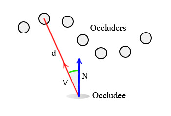
 Figure 4: The ideal sampling sphere for determining occlusion.
Of course, performing a complex 3D integration at every pixel of a rendered image is completely impractical. Instead, we will approximate this sphere by using a 3D sampling kernel that resides within the sphere's volume. The sampling kernel is then used to look into the depth buffer at the specified locations and determine if each of it's virtual points are obscured by the depth buffer surface. An example sampling kernel is shown in Figure 5, as well as how it would be applied to our surface point.
물론 렌더링된 이미지의 모든 픽셀에 대해 복잡한 3D 총합을 구하는 것은 완전히 실용적이지 못하다. 대신에 우리는 구의 볼륨이내에 상주하는 3D 샘플링 커널에 의해 이 구를 간략화 할 것이다. 샘플링 커널은 특정 위치에 있는 깊이 버퍼를 조사하고 각각의 가상의 점들이 깊이 버퍼 표면에 의해 가려졌는지 아닌지를 결정하는데 사용된다. 샘플링 커널의 한가지 예는 Figure5를 보고 우리 표면의 점에 어떻게 적용되는지를 보자.
 Figure 5: Simplified sampling kernel and its position on the depth buffer.
The occlusion factor can then be calculated as the sum of the sampling kernel point's individual occlusions. As you will see in the implementation section, these individual calculations can be made more or less sensitive based on several different factors, such as distance from the camera, the distance between our point and the occluding point, and artist specified scaling factors.
차폐 요소는 샘플링 커널 점들의 각각의 차폐된 정도의 함으로 계산할 수 있다. 구현 섹션을 보면 이 개별적인 계산은 카메라로 부터의 거리, 점과 차폐점사이의 거리, 아티스트들이 잡아줄 크기 요소등 몇가지 다른 요소들을 기반으로 감각적으로 만들 수 있다.
Implementation
With a clear understanding of how the algorithm functions, we can now discuss a working implementation. As discussed in the algorithm theory section, we will need a source of scene depth information. For simplicity's sake, we will use a separate floating point buffer to store the depth data. A more efficient technique, although slightly more complex, would utilize the z-buffer to acquire the scene depth. The following code snippet shows how to create the floating point buffer, as well as the render target and shader resource views that we will be binding it to the pipeline with:
알고리즘 함수의 확실한 이해를 통해 우리는 지금부터 구현에 대해 이야기해 볼 수 있다. 알고리즘 이론 섹션에서 이야기 했듯이, 우리는 씬의 깊이 정보의 소스를 필요로한다. 간단하게 깊이 정보를 저장하기 위해 별개의 부동소스점 버퍼를 사용할 것이다. 비록 약간 더 복잡할 수는 있겠지만 더 효율적인 기법은 씬의 깊이를 얻어오는데 z-buffer를 이용하는 것이다. 뒤의 코드는 어떻게 부동소수점 버퍼를 어떻게 생성하는지 보여주고 또한 우리 파이프라인에 연결시킬 렌더타겟과 쉐이더 리소스 뷰의 생성도 보여준다.
// Create the depth buffer
D3D10_TEXTURE2D_DESC desc;
ZeroMemory( &desc, sizeof( desc ) );

desc.Width = pBufferSurfaceDesc->Width;
desc.Height = pBufferSurfaceDesc->Height;
desc.MipLevels = 1;
desc.ArraySize = 1;
desc.Format = DXGI_FORMAT_R32_FLOAT;
desc.SampleDesc.Count = 1;
desc.Usage = D3D10_USAGE_DEFAULT;
desc.BindFlags = D3D10_BIND_RENDER_TARGET | D3D10_BIND_SHADER_RESOURCE;

pd3dDevice->CreateTexture2D( &desc, NULL, &g_pDepthTex2D );

// Create the render target resource view
D3D10_RENDER_TARGET_VIEW_DESC rtDesc;
rtDesc.Format = desc.Format;
rtDesc.ViewDimension = D3D10_RTV_DIMENSION_TEXTURE2D;
rtDesc.Texture2D.MipSlice = 0;

pd3dDevice->CreateRenderTargetView( g_pDepthTex2D, &rtDesc, &g_pDepthRTV );

// Create the shader-resource view
D3D10_SHADER_RESOURCE_VIEW_DESC srDesc;
srDesc.Format = desc.Format;
srDesc.ViewDimension = D3D10_SRV_DIMENSION_TEXTURE2D;
srDesc.Texture2D.MostDetailedMip = 0;
srDesc.Texture2D.MipLevels = 1;

pd3dDevice->CreateShaderResourceView( g_pDepthTex2D, &srDesc, &g_pDepthSRV );
Once the depth information has been generated, the next step is to calculate the occlusion factor at each pixel in the final scene. This information will be stored in a second single component floating point buffer. The code to create this buffer is very similar to the code used to create the floating point depth buffer, so it is omitted for brevity.
Now that both buffers have been created, we can describe the details of generating the information that will be stored in each of them. The depth buffer will essentially store the view space depth value. The linear view space depth is used instead of clip space depth to prevent any depth range distortions caused by the perspective projection. The view space depth is calculated by multiplying the incoming vertices by the worldview matrix. The view space depth is then passed to the pixel shader as a single component vertex attribute.
깊이 정보를 생성하고, 다음 스텝은 마지막 씬에 각각의 픽셀에 대해 차폐 요소를 계산하는 것이다. 이 정보는 부동소수점 버퍼에 두번째 단일 성분에 저장될 것이다. 이 버퍼를 생성하는 코드는 부동소스점 깊이 버퍼를 생성하는데 사용된 코드와 매우 유사하다. 그래서 글을 줄이기 위해 제외하였다.
이제 두 버퍼들의 생성되었고 우리는 각각에 저장될 정보를 생성하는 것에 대해 자세한 부분을 설명할 수 있다. 깊이 버퍼는 필수적으로 뷰 공간의 깊이값을 저장할 것이다. 원근 투영에 의해 발생될 수 있는 깊이 범위의 왜곡을 예방하기 위해 클립 공간의 깊이 대신에 선형 뷰 공간 깊이를 사용한다. 뷰 공간 깊이는 넘어온 버텍스에 월드-뷰 행렬을 곱해줌으로써 계산된다. 뷰 공간 깊이는 버텍스 속성의 단일 성분으로 픽셀 쉐이더로 넘어간다.
fragment VS( vertex IN )
{
    fragment OUT;

    // Output the clip space position
    OUT.position = mul( float4(IN.position, 1), WVP );

    // Calculate the view space position
    float3 viewpos = mul( float4( IN.position, 1 ), WV ).xyz;

    // Save the view space depth value
    OUT.viewdepth = viewpos.z;

    return OUT;
}
To store the depth values in the floating point buffer, we then scale the value by the distance from the near to the far clipping planes in the pixel shader. This produces a linear, normalized depth value in the range [0,1].
부동소수점 버퍼에 깊이 값을 저장하기 위해 우리는 픽셀 쉐이더에서 근단면에서 부터 원단면까지의 거리에 대해 값의 크기를 조정한다. 이것은 선형적이고 [0, 1]사이의 범위를 가지는 정규화된 깊이값을 생성한다.
pixel PS( fragment IN )
{
    pixel OUT;

    // Scale depth by the view space range
    float normDepth = IN.viewdepth / 100.0f;

    // Output the scaled depth
    OUT.color = float4( normDepth, normDepth, normDepth, normDepth );

    return OUT;
}
With the normalized depth information stored, we then bind the depth buffer as a shader resource to generate the occlusion factor for each pixel and store it in the occlusion buffer. The occlusion buffer generation is initiated by rendering a single full screen quad. The vertices of the full screen quad only have a single two-component attribute which specifies the texture coordinates at each of its four corners corresponding to their locations in the depth buffer. The vertex shader trivially passes these parameters through to the pixel shader.
정규화된 깊이 정보를 저장하고, 각각의 픽셀의 차폐 요소를 생성하고 차폐 버퍼에 저장하기 위해 쉐이더 리소스로 깊이 버퍼를 연결한다. 이 차폐 버퍼 생성은 하나의 풀 스크린을 덮는 사각형 하나를 렌더링 하는것에 의해 시작된다. 풀 스크린 사각형의 버텍스들은 깊이 버퍼에 위치에 대응되는 4개의 코너 각각의 텍스쳐 좌표를 명시하는 단일 2차원 성분만 가진다. 버텍스 쉐이더는 평범하게 이 파라미터들을 픽셀 쉐이더로 넘겨준다.
fragment VS( vertex IN )
{
    fragment OUT;

    OUT.position = float4( IN.position.x, IN.position.y, 0.0f, 1.0f );
    OUT.tex = IN.tex;

    return OUT;
}
The pixel shader starts out by defining the shape of the 3D sampling kernel in an array of three component vectors. The lengths of the vectors are varied in the range [0,1] to provide a small amount of variation in each of the occlusion tests.
픽셀 쉐이더는 3차원 벡터의 배열에 3D 샘플링 커널의 모양을 정의함으로써 시작한다. 벡터의 길이는 [0, 1] 범위에서 차폐 테스트의 각각 변화의 작은 값들을 생성하기 위해 다양하게 만든다.
const float3 avKernel[8] =
{
    normalize( float3( 1, 1, 1 ) ) * 0.125f,
    normalize( float3( -1,-1,-1 ) ) * 0.250f,
    normalize( float3( -1,-1, 1 ) ) * 0.375f,
    normalize( float3( -1, 1,-1 ) ) * 0.500f,
    normalize( float3( -1, 1 ,1 ) ) * 0.625f,
    normalize( float3( 1,-1,-1 ) ) * 0.750f,
    normalize( float3( 1,-1, 1 ) ) * 0.875f,
    normalize( float3( 1, 1,-1 ) ) * 1.000f
};
Next, the pixel shader looks up a random vector to reflect the sampling kernel around from a texture lookup. This provides a high degree of variation in the sampling kernel used, which will allow us to use a smaller number of occlusion tests to produce a high quality result. This effectively "jitters" the depths used to calculate the occlusion, which hides the fact that we are under-sampling the area around the current pixel.
다음으로, 픽셀 쉐이더는 텍스쳐 룩업으로 부터 샘플링 커널을 반사시키기 위한 랜덤 벡터를 얻어온다. 이것은 샘플링 커널 사용에 대단한 변화를 제공하여 높은 품질의 결과를 생성하기 위한 차폐 테스트의 횟수를 더 줄여줄 것이다. 깊이의 효과적인 "jitters"는 현재 픽셀 주변에 영역에 더 낮게 샘플링되는 요소를 숨기면서 차폐를 계산하는데 사용된다.
float3 random = VectorTexture.Sample( VectorSampler, IN.tex.xy * 10.0f ).xyz;

random = random * 2.0f - 1.0f;
Now the pixel shader will calculate a scaling to apply to the sampling kernel based on the depth of the current pixel. The pixel's depth value is read from the depth buffer and expanded back into view space by multiplying by the near to far clip plane distance. Then the scaling for the x and y component of the sampling kernel are calculated as the desired radius of the sampling kernel (in meters) divided by the pixel's depth (in meters). This will scale the texture coordinates used to look up individual samples. The z component scale is calculated by dividing the desired kernel radius by the near to far plane distance. This allows all depth comparisons to be performed in the normalized depth space that our depth buffer is stored in.
이제 픽셀 쉐이더는 현재 픽셀의 깊이에 기반하여 샘플링 커널을 적용하기 위해 크기를 계산할 것이다. 이 픽셀들의 깊이 값은 깊이 버퍼에서 읽어오고 근단면, 원단면의 거리에 의해 곱해짐으로써 뷰 공간으로 확장된다. 샘플링 커널의 x, y 성분의 크기는 샘플링 커널의 원하는 반지름 크기(미터단위)를 픽셀의 깊이(미터단위)로 나눈 값으로 계산된다. 이것은 개별적인 샘플들을 찾는데 사용될 텍스쳐 좌표의 크기를 변경시킬 것이다. z 성분의 크기는 희망하는 커널 반지름을 근단면, 원단면 거리차로 나는 값으로 계산된다. 이것은 우리의 깊이 버퍼를 저장한 정규화된 깊이 공간에 행해지는 모든 깊이 비교를 가능하게한다.
float fRadius = vSSAOParams.y;
float fPixelDepth = DepthTexture.Sample( DepthSampler, IN.tex.xy ).r;
float fDepth = fPixelDepth * vViewDimensions.z;
float3 vKernelScale = float3( fRadius / fDepth, fRadius / fDepth, fRadius / vViewDimensions.z ) ;
With the kernel scaling calculated, the individual occlusion tests can now be carried out. This is performed in a for loop which iterates over each of the points in the sampling kernel. The current pixel's texture coordinates are offset by the randomly reflected kernel vector's x and y components and used to look up the depth at the new location. This depth value is then offset by the kernel vector's z-component and compared to the current pixel depth.
커널 샘플링을 계산하면서 개별적인 차폐 테스트는 바로 수행될 수 있다. 이것은 샘플링 커널의 각 점들을 도는 루프에서 행해진다. 현재 픽셀의 텍스쳐 좌표는 커널 벡터의 x, y 성분을 랜덤하게 반사시킨 만큼 옮겨지고 새로운 위치의 깊이값을 찾는데 사용된다. 이 깊이 값은 커널 벡터의 z 성분만큼 옮겨지고 현재 픽셀 깊이와 비교된다.
float fOcclusion = 0.0f;
for ( int j = 1; j < 3; j++ )
{
float3 random = VectorTexture.Sample( VectorSampler, IN.tex.xy * ( 7.0f + (float)j ) ).xyz;
random = random * 2.0f - 1.0f;
for ( int i = 0; i < 8; i++ )
{
float3 vRotatedKernel = reflect( avKernel[i], random ) * vKernelScale;
float fSampleDepth = DepthTexture.Sample( DepthSampler, vRotatedKernel.xy + IN.tex.xy ).r;
float fDelta = max( fSampleDepth - fPixelDepth + vRotatedKernel.z, 0 );
float fRange = abs( fDelta ) / ( vKernelScale.z * vSSAOParams.z );
fOcclusion += lerp( fDelta * vSSAOParams.w, vSSAOParams.x, saturate( fRange ) );
}
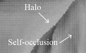
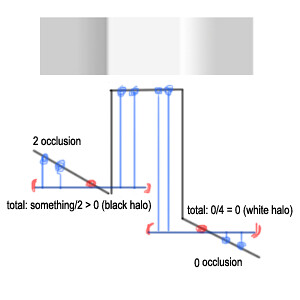
}The delta depth value is then normalized by an application selectable range value. This is intended to produce a factor to determine the relative magnitude of the depth difference. This information can, in turn, be used to adjust the influence of this particular occlusion test. For example, if an object is in the foreground of a scene, and another object is partially obscured behind it then you don't want to count a failed occlusion test for the back object if the foreground object is the only occluder. Otherwise the background object will show a shadow-like halo around the edges of the foreground object. The implementation of this scaling is to linearly interpolate between a scaled version of the delta value and a default value, with the interpolation amount based on the range value.
델타 깊이 값은 어플리케이션에서 선택한 범위 값에 의해 정규화된다. 이것은 깊이 차이의 상대적인 크기를 결정하는 요소를 생산하기 위한 의도이다. 결국 이 정보는 이 특정한 차폐 테스트의 정도(영향)을 조절하는데 사용될 수 있다. 예를 들어 만약 하나의 오브젝트가 씬의 앞부분에 있고 다른 한 물체는 이 물체의 뒤에서 부분적으로 가려졌다면 앞에 있는 오브젝트가 유일한 차폐물이라면 뒤에 있는 오브젝트에 대한 실패할 차폐 테스트를 하는걸 원하진 않을 것이다. 반면에 뒤에 있는 오브젝트는 앞의 물체의 가장자리 주변에 후광과 같은 그림자가 보일것이다. 이 크기의 구현은 델타 값의 크기가 변경된 것과 기본 값 사이의 범위 값을 기반으로한 선형 보간으로 구현된다.
fOcclusion += lerp( ( fDelta * vSSAOParams.w ), vSSAOParams.x, saturate( fRange ) );
The final step before emitting the final pixel color is to calculate an average occlusion value from all of the kernel samples, and then use that value to interpolate between a maximum and minimum occlusion value. This final interpolation compresses the dynamic range of the occlusion and provides a somewhat smoother output. It should also be noted that in this chapter’s demo program, only sixteen samples are used to calculate the current occlusion. If a larger number of samples are used, then the occlusion buffer output can be made smoother. This is a good place to scale the performance and quality of the algorithm for different hardware levels.
최종 픽셀 색을 내보내기 전에 마지막 단계는 모든 커널 샘플들의 평균 차폐 값을 계산하고 최대, 최소 차폐 값 사이로 보간하기 위한 값으로 사용하는 것이다. 이 마지막 보간은 차폐의 동적인 범위를 압축하고 더 부드러운 결과물을 제공한다. 또한 이 챕터의 데모 프로그램안에서 적혀있듯이 오직 16개 샘플들이 현재 차폐 계산에 사용되었다. 만약 더 큰 숫자의 샘플들을 사용한다면, 차폐 버퍼 결과물은 더 부드럽게 될 것이다. 이것은 다른 하드웨어 레벨에서 알고리즘의 퍼포먼스와 질을 키우는데 좋은 지점이 된다.
OUT.color = fOcclusion / ( 2.0f * 8.0f );

// Range remapping
OUT.color = lerp( 0.1f, 0.6, saturate( OUT.color.x ) );
With the occlusion buffer generated, it is bound as a shader resource to be used during the final rendering pass. The rendered geometry simply has to calculate it's screen space texture coordinates, sample the occlusion buffer, and modulate the ambient term by that value. The sample file provided performs a simple five sample average, but more sophisticated filtering like a Gaussian blur could easily be used instead.
차폐 버퍼를 생성하면서 마지막 렌더링 패스 동안 사용되기 위해 쉐이더 리소스로 넘겼다. 렌더링된 지오메트리는 간단하게 화면 공간 텍스쳐 좌표로 계산하고 차폐 버퍼에 샘플링하고 그 값에 의해 환경값을 조절한다. 샘플 파일은 간단한 다섯 샘플을 평균내서 처리하지만 가우시안 블러와 같은 더 세련된 필터링은 쉽게 대신 사용될 수 있다.
SSAO Demo
Demo Download: SSAO_Demo
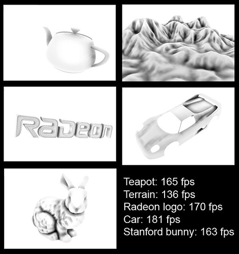
The demo program developed for this chapter provides a simple rendering of a series of cube models that is shaded only with our screen space ambient occlusion. The adjustable parameters discussed for this technique can be changed in real-time with the onscreen slider controls. Figure 6 below shows the occlusion buffer and the resulting final output rendering. Notice that the occlusion parameters have been adjusted to exaggerate the occlusion effect.
이 챕터를 위해 개발된 데모 프로그램은 우리 SSAO만으로 쉐이딩을 계산하는 큐브 모델들을 간단하게 랜더링한다. 이 기법에서 의논된 조정할만한 파라미터들은 화면상의 슬라이더 컨트롤로 실시간에 변경할 수 있다. 뒤의 Figure 6은 차폐 버퍼와 최종 결과물 렌더링을 보여준다. 차폐 파라미터들은 차폐 효과를 과장하기 위해 조정되어 진다는 것을 알아두자.
 Figure 6: A sample ambient occlusion buffer from the demo program.
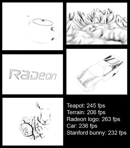
 Figure 7: The final output rendering from the demo program.
Conclusion
In this chapter we developed an efficient, screen space technique for adding realism to the ambient lighting term of the standard phong lighting model. This technique provides one implementation of the SSAO algorithm, but it is certainly not the only one. The current method can be modified for a given type of scene, with more or less occlusion for distant geometry. In addition, the minimum and maximum amounts of occlusion, interpolation techniques, and sampling kernels are all potential areas for improvement or simplification. This chapter has attempted to provide you with an insight into the inner workings of the SSAO technique as well as a sample implementation to get you started.
이번 챕터에서 우리는 표준 퐁 라이팅 모델에 환경 광 개념으로 사실성을 추가하기 위한 효율적인 화면 공간 기법을 개발해봤다. 이 기법은 SSAO 알고리즘의 한가지 구현을 제공하지만 딱 이것 하나만은 아니다. 현재 메소드는 씬의 주어진 타입에 맞춰 수정될 수 있고 지오메트리의 거리에 따라 더 혹은 덜 차폐를 계산할 수 있다. 게다가 차폐의 최소, 최대 값, 보간, 샘플링 커널은 모두 더 향상시키거나 간략화 할 수있는 부분이다. 이 챕터는 당신에게 SSAO 기법의 내부 동작에 대한 시야와 샘플 구현을 시작하는 것을 돕기 위해 만들어졌다.